If you’ve worked with ML models long enough, you’ve probably run into this situation: your model gives a prediction, and you have no idea how much to trust it.

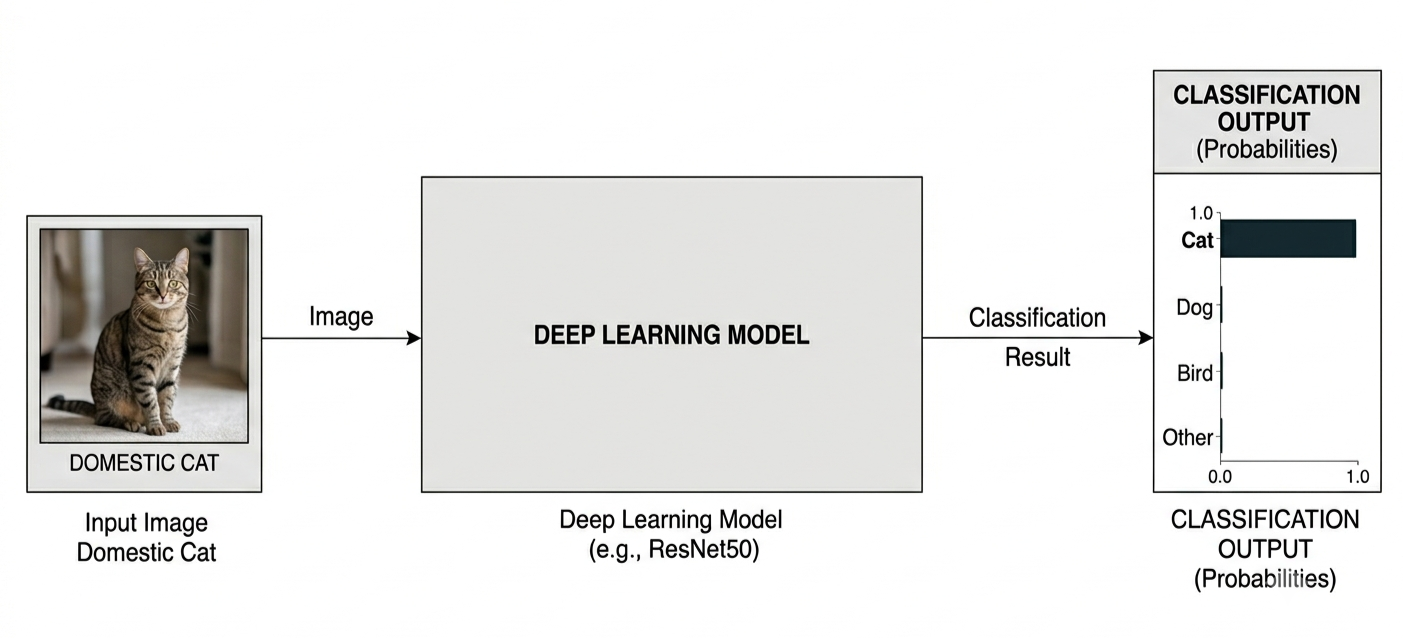
The model says “cat”, but is it 99% sure or 1% sure? And even if it gives you a probability, how do you know that probability is actually calibrated?

Conformal prediction offers a way out. It’s a framework that takes any pre-trained model and wraps it with a coverage guarantee, without retraining, without assumptions about how your model works internally, and without assumptions about the distribution of your data.

Specifically, it guarantees that the correct answer will be in the prediction set at least $(1 - \alpha)$ of the time, where $\alpha$ is a threshold you choose yourself.

In this post we’ll build up the intuition behind why this works, walk through the proof, and implement it from scratch in Python with experiments to verify the guarantee holds.

Conformal Prediction

Conformal prediction was introduced by Vladimir Vovk, Alexander Gammerman, and Glenn Shafer in the late 1990s, and formalized in their 2005 book Algorithmic Learning in a Random World. The version we use today, split conformal prediction, was introduced by Papadopoulos et al. in Inductive Confidence Machines for Regression, which made it practical for real pipelines. A more accessible introduction is A Gentle Introduction to Conformal Prediction by Angelopoulos & Bates.

The key insight is simple: instead of giving a single prediction, the model gives a set of predictions. This set comes with a formal guarantee that the correct answer will be inside it at least $(1 - \alpha)$ of the time.

There are three ingredients: a calibration set of labeled examples, a conformity score that measures how surprised the model is by the correct answer, and a threshold $\lambda$ computed from those scores. At test time, any label whose score falls below $\lambda$ goes into the prediction set.

Here’s an example:

Say we have a classifier that takes an image and outputs a probability for each class: cat, dog, fox, wolf. For each example in our calibration set, we compute the conformity score:

s = 1 - P(correct class)

So if the model gives 0.80 probability to the correct class, the score is 0.20 (low surprise). If it gives 0.15, the score is 0.85 (high surprise).

Say we have n = 5 calibration examples with these scores:

Image	Correct Label	Model Confidence	Score s
Image 1	cat	0.90	0.10
Image 2	dog	0.75	0.25
Image 3	fox	0.60	0.40
Image 4	cat	0.55	0.45
Image 5	dog	0.30	0.70

Sorted scores: 0.10, 0.25, 0.40, 0.45, 0.70

We choose α = 0.20, meaning we want the correct answer in our prediction set at least 80% of the time. The threshold is computed as:

λ = the ⌈(n+1)(1-α)⌉th smallest score = ⌈6 × 0.80⌉ = 5th smallest = 0.70

Now a new image arrives. The model outputs:

Label	Confidence	Score
cat	0.60	0.40
dog	0.25	0.75
fox	0.10	0.90
wolf	0.05	0.95

We include every label with score ≤ 0.70. That gives us {cat} as our prediction set.

If the model were less confident, say it spread probabilities more evenly, more labels would fall below λ and the set would grow to something like {cat, dog}. The set size reflects the model’s uncertainty.

Proof

The guarantee conformal prediction makes is:

Recall how we build the prediction set: we include a label $y$ if its conformity score is below $\lambda$. So the correct answer $Y_{n+1}$ is in the prediction set if and only if:

And it is excluded when $s(X_{n+1}, Y_{n+1}) > \lambda$. So the guarantee reduces to showing:

Exchangeability

The proof rests on one assumption: the calibration points and the test point are all random draws from the same population. This is called exchangeability. It means no single point is special: if you took all $n+1$ points and shuffled their order randomly, the joint distribution wouldn’t change.

A simple way to think about it: imagine all $n+1$ conformity scores written on identical slips of paper and placed in a bag. You draw $n$ of them for calibration and leave one in the bag. That remaining slip, the test score, is no different from any of the ones you drew. It’s just another random slip from the same bag.

The Rank Argument

Because of exchangeability, the test score is equally likely to be at any rank among all $n+1$ scores. Let’s make this concrete with our earlier example.

We had 5 calibration scores: 0.10, 0.25, 0.40, 0.45, 0.70. Now say the test score turns out to be 0.35. The full sorted list of all 6 scores is:

0.10, 0.25, 0.35, 0.40, 0.45, 0.70

The test score lands at rank 3 out of 6. But before we observe it, it was equally likely to land at any of the 6 ranks, each with probability 1/6.

We set $\lambda = 0.70$, the 5th smallest score. The test score falls below $\lambda$ when it lands at ranks 1, 2, 3, 4, or 5, any rank except the very top. That’s 5 out of 6 possible ranks:

And our target was $1 - \alpha = 1 - 0.20 = 0.80$. So $0.833 \geq 0.80$

In general, $\lambda$ is chosen as the $\lceil(n+1)(1-\alpha)\rceil$th smallest score, so:

That’s the entire proof. No assumptions about the model, no assumptions about the data distribution. Just exchangeability and a counting argument about ranks.

Implementation from Scratch

Let’s implement conformal prediction in python, using numpy and sklearn for the base classifier.

First, let’s generate a synthetic dataset. We’ll create a simple 3-class classification problem:

import numpy as np
import matplotlib.pyplot as plt
from sklearn.datasets import make_classification
from sklearn.model_selection import train_test_split
from sklearn.neural_network import MLPClassifier

# Generate synthetic data
X, y = make_classification(
    n_samples=2000,
    n_features=10,
    n_classes=3,
    n_informative=5,
    random_state=42
)

# Split into train, calibration, test
X_train, X_temp, y_train, y_temp = train_test_split(X, y, test_size=0.4, random_state=42)
X_cal, X_test, y_cal, y_test = train_test_split(X_temp, y_temp, test_size=0.5, random_state=42)

print(f"Train size: {len(X_train)}")
print(f"Calibration size: {len(X_cal)}")
print(f"Test size: {len(X_test)}")

# Train a simple classifier
model = MLPClassifier(hidden_layer_sizes=(64, 32), random_state=42, max_iter=500)
model.fit(X_train, y_train)
print(f"Model accuracy: {model.score(X_test, y_test):.3f}")

Next, we compute conformity scores on the calibration set and find the threshold $\lambda$:

def get_conformity_scores(model, X, y):
    """
    Conformity score = 1 - P(correct class)
    Low score = model was confident about the right answer
    High score = model was surprised
    """
    probs = model.predict_proba(X)
    correct_class_probs = probs[np.arange(len(y)), y]
    return 1 - correct_class_probs

def get_lambda(cal_scores, alpha):
    """
    Find the threshold λ = the ⌈(n+1)(1-α)⌉th smallest calibration score
    """
    n = len(cal_scores)
    rank = int(np.ceil((n + 1) * (1 - alpha)))
    rank = min(rank, n)  # cap at n in case of rounding
    sorted_scores = np.sort(cal_scores)
    return sorted_scores[rank - 1]

# Compute calibration scores and find λ
alpha = 0.1  # we want 90% coverage
cal_scores = get_conformity_scores(model, X_cal, y_cal)
lam = get_lambda(cal_scores, alpha)

print(f"λ = {lam:.3f}")

One thing worth noting: the min(rank, n) line. When $\alpha$ is very small, say 0.01, the formula $\lceil(n+1)(1-\alpha)\rceil$ can produce a rank larger than $n$. For example with $n = 100$ and $\alpha = 0.01$:

That’s fine. But with $n = 99$ and $\alpha = 0.005$:

We only have 99 calibration scores, so rank 100 doesn’t exist and this would throw an index error. Capping at $n$ means that in these edge cases we just return the largest calibration score as $\lambda$, which is the most conservative choice. The coverage guarantee still holds.

Now we build prediction sets:

def get_prediction_sets(model, X, lam):
    """
    For each input, include all labels whose conformity score is below λ
    """
    probs = model.predict_proba(X)
    # A label is included if 1 - P(label) <= λ
    # Which is equivalent to P(label) >= 1 - λ
    prediction_sets = probs >= (1 - lam)
    return prediction_sets

# Build prediction sets for the test set
prediction_sets = get_prediction_sets(model, X_test, lam)

# Each row is a boolean array — True means the label is included
# Let's look at a few examples
for i in range(5):
    included_labels = np.where(prediction_sets[i])[0]
    print(f"Test point {i}: prediction set = {included_labels}, true label = {y_test[i]}")

Now let’s verify the guarantee actually holds on our test set:

def compute_coverage(prediction_sets, y_test):
    """
    Coverage = fraction of test points where the true label is in the prediction set
    """
    covered = prediction_sets[np.arange(len(y_test)), y_test]
    return covered.mean()

coverage = compute_coverage(prediction_sets, y_test)
print(f"Target coverage: {1 - alpha:.2f}")
print(f"Empirical coverage: {coverage:.3f}")

Target coverage: 0.90
Empirical coverage: 0.943

The empirical coverage clears the target.

Does the coverage guarantee hold across α?

Let’s verify the guarantee holds across a range of $\alpha$ values:

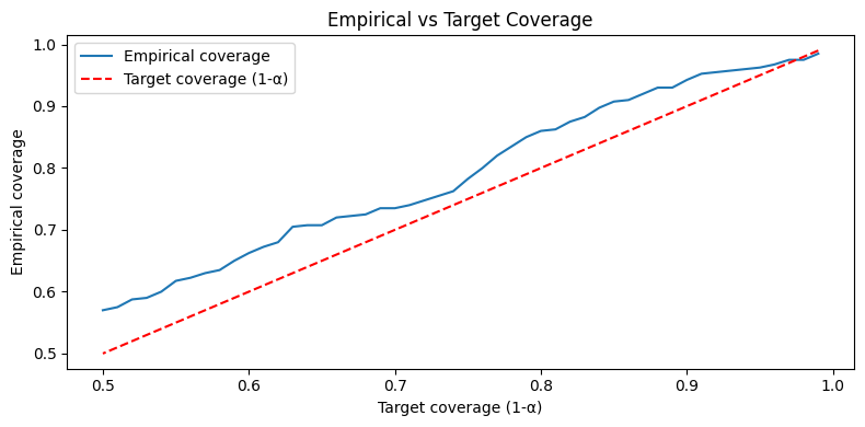
And how does prediction set size change with $\alpha$?

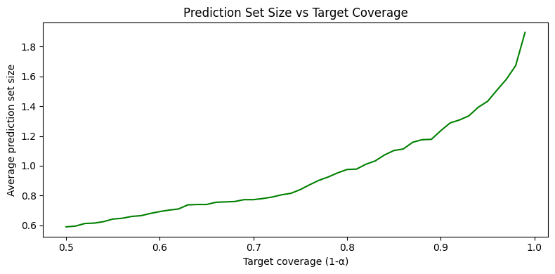
As target coverage increases, prediction sets grow larger: the model has to cast a wider net to keep the correct answer included. When the model is confident, sets stay small even at high coverage. When it’s uncertain, sets grow. Uncertainty is reflected directly in the set size.

Caveats

Conformal prediction comes with a couple of caveats worth knowing.

• Exchangeability must hold. The guarantee relies entirely on the assumption that calibration and test points come from the same population. Under distribution shift, it breaks.

• It’s an average guarantee, not an individual one. The coverage guarantee says the correct answer is in the prediction set at least $(1 - \alpha)$ of the time on average across many test points. It says nothing about any specific individual prediction.