Deriving the ELBO: The Loss Function Behind Variational Autoencoders
If you’ve ever trained a Variational Autoencoder (VAE), you’ve used the ELBO — the Evidence Lower BOund — whether you noticed it or not. It’s the loss you minimize: a reconstruction term plus a KL term. In this post I want to derive it from scratch, starting from a plain autoencoder and using nothing beyond basic probability. By the end, those two familiar terms fall out of the math on their own.
From Autoencoders to Generative Models
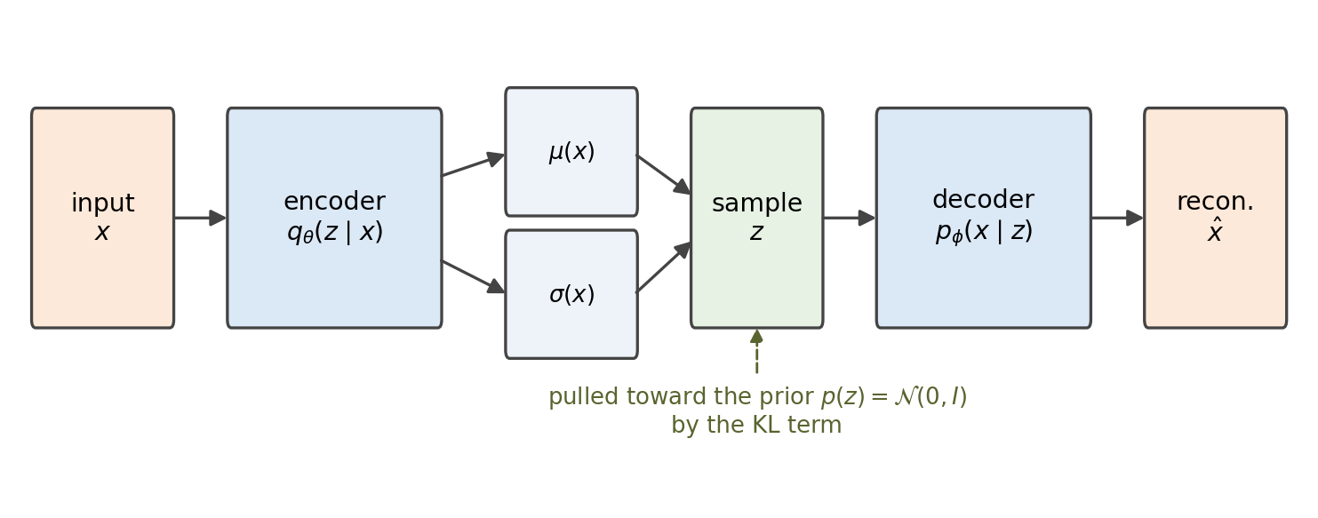
A standard autoencoder (AE) learns two functions: an encoder that compresses an input $x$ (say, a $28 \times 28$ MNIST digit) into a small latent vector $z$, and a decoder that reconstructs $x$ from $z$. It’s trained purely to minimize reconstruction error.
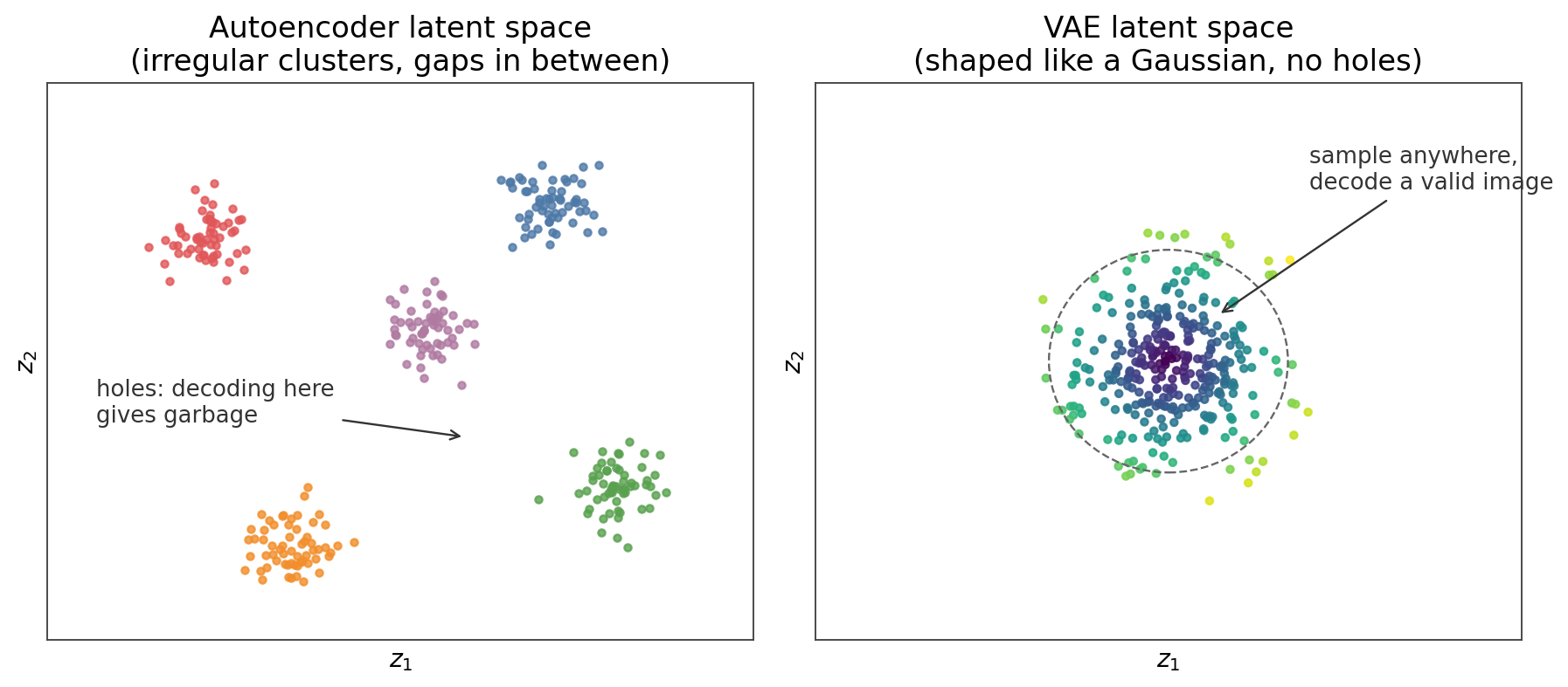
This works great for compression, but it fails as a generative model. If you pick a random point in the latent space and decode it, you usually get garbage. Why? Because the AE was never asked to organize its latent space. The encodings of real images end up as scattered islands, with large empty holes between them. The decoder has only ever seen the islands, so it has no idea what to do with the holes.
What we want instead is a latent space with two properties:
- No holes. Every point we might sample should decode to a plausible image. A natural way to enforce this is to make the latent codes follow a known, simple distribution, like a standard Gaussian $\mathcal{N}(0, I)$. Then generating a new image is trivial: sample $z \sim \mathcal{N}(0, I)$, decode it.
- Smoothness. Points that are close together in latent space should decode to similar images, so that moving through the space morphs one image into another continuously.
The VAE gives us both. To see how, we have to stop thinking about reconstruction for a moment and think about probabilities instead.
What We Actually Want: $p(x)$
Think of our dataset as samples from some unknown data-generating process. For an image $x \in \mathbb{R}^{28 \times 28}$,
\[p(x) = \text{the probability that the data-generating process produces exactly this image.}\]A good generative model assigns high probability to real images and low probability to noise. So training a generative model means one thing: maximize $p(x)$ for the images in our training set.
There’s just one problem. $x$ lives in a 784-dimensional pixel space, and modeling the joint distribution over 784 pixels directly is hopeless. The pixels are correlated in complicated ways — a “7” isn’t a bag of independent pixel values.
Enter the Latent Variable $z$
Here’s the key modeling assumption: images aren’t created pixel by pixel. They’re created from a much smaller hidden description.
Think of $z$ as a recipe. For a digit, the recipe might encode something like “it’s a 7, slanted slightly left, thin stroke, written near the top.” The generative machine works in two steps:
- It picks a recipe $z$. The probability of picking a particular recipe is $p(z)$, the prior.
- Given that recipe, it produces an image. The probability of producing image $x$ from recipe $z$ is $p(x \mid z)$, the likelihood (this will be our decoder).
So what is $p(x, z)$? It’s the probability that both things happen: the machine picks recipe $z$ and produces image $x$ from it. The chain rule of probability says $P(A, B) = P(A) \cdot P(B \mid A)$. With event $A$ = “choosing $z$” and event $B$ = “generating $x$”:
\[p(x, z) = p(z)\, p(x \mid z)\]In words: the probability of choosing latent $z$, times the probability of generating $x$ given that $z$. This factorization is the reason we introduce $z$ in the first place. Each piece is simple ($p(z)$ is just a Gaussian, $p(x \mid z)$ is a neural network), even though $p(x)$ itself is complicated.
Recovering $p(x)$: Marginalization
We have $p(x, z)$, but we wanted $p(x)$. How do we get rid of $z$?
Forget the infinitely many possible latent vectors for a second, and imagine there are only three possible recipes: $z_1$, $z_2$, $z_3$. What’s the probability of seeing a particular image $x$? There are exactly three mutually exclusive ways it could have happened:
- The model chose $z_1$, then generated $x$.
- The model chose $z_2$, then generated $x$.
- The model chose $z_3$, then generated $x$.
Since these are the only possibilities and they can’t co-occur, we add their probabilities:
\[p(x) = p(x, z_1) + p(x, z_2) + p(x, z_3) = \sum_i p(x, z_i)\]In reality $z$ is continuous, so the sum becomes an integral:
\[p(x) = \int p(x, z)\, dz = \int p(z)\, p(x \mid z)\, dz\]And this is where we get stuck. The integral is over every possible latent vector. For a 32-dimensional latent space, that’s an integral over all of $\mathbb{R}^{32}$ with a neural network sitting inside it. It’s intractable. We can’t compute $p(x)$, so we can’t directly maximize it.
The Posterior, and Why We Approximate It
Bayes’ rule tells us the distribution over recipes given an image, the posterior:
\[p(z \mid x) = \frac{p(x, z)}{p(x)}\]This is exactly what an encoder should compute: given this image, which recipes could have produced it? But look at the denominator. It’s the same intractable $p(x)$. So the true posterior $p(z \mid x)$ is out of reach too.
The variational trick is this: since we can’t compute $p(z \mid x)$, we approximate it with a distribution we can work with. We introduce
\[q_\theta(z \mid x) \approx p(z \mid x)\]where $q_\theta$ is a Gaussian $\mathcal{N}!\left(\mu_\theta(x),\, \sigma_\theta(x)\right)$ whose mean and variance are predicted by a neural network with parameters $\theta$. This network is the encoder.
One clarification that trips a lot of people up: the distributions we choose to be Gaussian are the prior $p(z) = \mathcal{N}(0, I)$ and the family of $q_\theta$. The true posterior $p(z \mid x)$ is not something we choose. It’s unknown and intractable, and it’s the target that $q_\theta$ tries to match. We pick Gaussians for $p(z)$ and $q_\theta$ because they’re easy to sample from, and because the KL divergence between two Gaussians has a clean closed form.
So we now have two distributions over $z$ given $x$:
- $q_\theta(z \mid x)$, the approximation predicted by our encoder,
- $p(z \mid x)$, the true (intractable) posterior, our target.
The standard way to measure how far apart two distributions are is the KL divergence, and we want to minimize it:
\[D_{KL}\!\left(q_\theta(z \mid x)\,\|\,p(z \mid x)\right) = \sum_{z \in \mathcal{Z}} q_\theta(z \mid x)\, \log \frac{q_\theta(z \mid x)}{p(z \mid x)}\](I’ll write sums over $z$ for readability. For continuous $z$, every $\sum_z$ is really an $\int dz$, and nothing in the derivation below changes.)
This looks like a dead end, since the KL contains $p(z \mid x)$, which we just said we can’t compute. But watch what happens when we expand it.
The Derivation
Step 1: substitute Bayes’ rule. Replace $p(z \mid x)$ with $\frac{p(x,z)}{p(x)}$:
\[D_{KL}\!\left(q_\theta(z \mid x)\,\|\,p(z \mid x)\right) = \sum_{z} q_\theta(z \mid x)\, \log \frac{q_\theta(z \mid x)\, p(x)}{p(x, z)}\]Step 2: split the log. Using $\log(ab) = \log a + \log b$:
\[= \sum_{z} q_\theta(z \mid x)\, \log \frac{q_\theta(z \mid x)}{p(x, z)} \;+\; \sum_{z} q_\theta(z \mid x)\, \log p(x)\]Step 3: pull out the constant. $\log p(x)$ doesn’t depend on $z$, so it comes out of the second sum:
\[= \sum_{z} q_\theta(z \mid x)\, \log \frac{q_\theta(z \mid x)}{p(x, z)} \;+\; \log p(x) \underbrace{\sum_{z} q_\theta(z \mid x)}_{=\,1}\]The probabilities of a distribution sum to 1, so:
\[D_{KL}\!\left(q_\theta(z \mid x)\,\|\,p(z \mid x)\right) = \sum_{z} q_\theta(z \mid x)\, \log \frac{q_\theta(z \mid x)}{p(x, z)} \;+\; \log p(x)\]Step 4: rearrange. Move things around to isolate $\log p(x)$ (flipping the fraction inside the log flips its sign, which is why the first term now adds instead of subtracts):
\[\log p(x) = \underbrace{\sum_{z} q_\theta(z \mid x)\, \log \frac{p(x, z)}{q_\theta(z \mid x)}}_{\text{call this } \mathcal{L}} \;+\; D_{KL}\!\left(q_\theta(z \mid x)\,\|\,p(z \mid x)\right)\]Step 5: use the one fact everyone knows about KL. KL divergence is always non-negative: $D_{KL} \geq 0$. Since it’s a non-negative term added to $\mathcal{L}$:
\[\log p(x) \;\geq\; \sum_{z} q_\theta(z \mid x)\, \log \frac{p(x, z)}{q_\theta(z \mid x)} \;=\; \mathcal{L}\]And there’s our bound. $\mathcal{L}$ is a lower bound on $\log p(x)$, the log-evidence. Hence the name: Evidence Lower BOund, ELBO. Unlike $\log p(x)$ itself, the ELBO contains only things we can compute: $q_\theta$ (our encoder) and $p(x, z) = p(z)\, p_\phi(x \mid z)$ (a fixed Gaussian prior and our decoder).
Why Maximizing the ELBO Is the Right Move
Look again at the identity from Step 4:
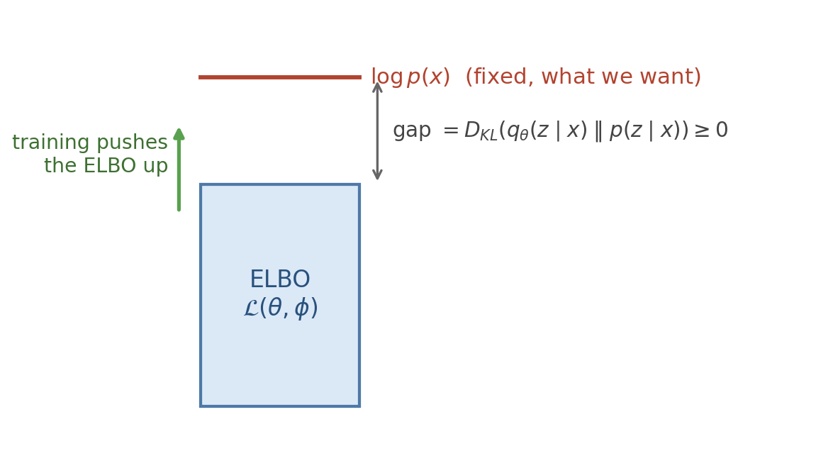
\[\log p(x) = \mathcal{L} + \underbrace{D_{KL}\!\left(q_\theta(z \mid x)\,\|\,p(z \mid x)\right)}_{\text{the gap}}\]For a fixed model, $\log p(x)$ is a fixed number, and the ELBO sits below it. The gap between them is exactly the KL divergence we originally wanted to minimize but couldn’t compute directly.
So maximizing the ELBO does two good things at once:
- It pushes up a lower bound on $\log p(x)$, making our model assign higher probability to real data. That’s the generative goal.
- It squeezes the gap, driving $q_\theta(z \mid x)$ toward the true posterior $p(z \mid x)$, making our encoder a better approximate-inference machine.
We turned an impossible objective (maximize an intractable integral) into a tractable one, and the price we pay is only that we optimize a lower bound instead of the true quantity.
Splitting the ELBO into the Two Familiar Terms
One last manipulation. Factor the joint inside the ELBO using $p(x, z) = p(z)\, p_\phi(x \mid z)$, where $p_\phi(x \mid z)$ is the decoder with parameters $\phi$:
\[\mathcal{L} = \sum_{z} q_\theta(z \mid x)\, \log \frac{p(z)\, p_\phi(x \mid z)}{q_\theta(z \mid x)}\]Split the log into two sums:
\[\mathcal{L} = \underbrace{\sum_{z} q_\theta(z \mid x)\, \log \frac{p(z)}{q_\theta(z \mid x)}}_{=\; -\,D_{KL}\left(q_\theta(z \mid x)\,\|\,p(z)\right)} \;+\; \underbrace{\sum_{z} q_\theta(z \mid x)\, \log p_\phi(x \mid z)}_{=\; \mathbb{E}_{z \sim q_\theta}\left[\log p_\phi(x \mid z)\right]}\]The first term is minus a KL divergence, but notice it’s a different KL than the one we started with. It compares the encoder’s output to the prior $p(z)$, not to the intractable posterior. Both are Gaussians we know, so this term has a closed-form formula. The second term is an expectation under $q_\theta$, which we estimate by sampling: encode $x$, sample a $z$, and score how well the decoder reconstructs $x$ from it. Putting it together:
\[\boxed{\;\mathcal{L} \;=\; \underbrace{\mathbb{E}_{z \sim q_\theta(z \mid x)}\!\left[\log p_\phi(x \mid z)\right]}_{\text{reconstruction term}} \;-\; \underbrace{D_{KL}\!\left(q_\theta(z \mid x)\,\|\,p(z)\right)}_{\text{regularization term}} \;\leq\; \log p(x)\;}\]Here’s what the two terms are saying:
- The reconstruction term says latents sampled from the encoder should let the decoder reproduce the input well. This is the old autoencoder objective in probabilistic form.
- The regularization term says the encoder’s distribution for every image should stay close to $\mathcal{N}(0, I)$. This is what fills the holes. It packs all the encodings into one smooth Gaussian blob, which is exactly the latent space we wanted at the start.
In practice, deep learning frameworks minimize losses, so the VAE loss is just the negative ELBO: reconstruction error plus a KL penalty. The two-term loss you write in code is this boxed equation with a minus sign in front.
One last thing worth noticing: nowhere in the derivation did we use anything specific to images, Gaussians, or neural networks. The bound $\mathcal{L} \leq \log p(x)$ holds for any choice of the approximating distribution $q(z \mid x)$. That generality is why the same ELBO shows up well beyond VAEs, in variational inference broadly, and even in diffusion models.
To actually train this with gradient descent, one more idea is needed: sampling $z$ isn’t differentiable, which is solved by the reparameterization trick. That deserves its own post.
References
- Kingma & Welling, Auto-Encoding Variational Bayes (2013), the original VAE paper.
- Kingma & Welling, An Introduction to Variational Autoencoders (2019), a longer, gentler treatment.