Visualizing Distribution Change in Forward Diffusion Process
Experiment: Visualizing Distribution Change
Experiment: Visualizing Distribution Change
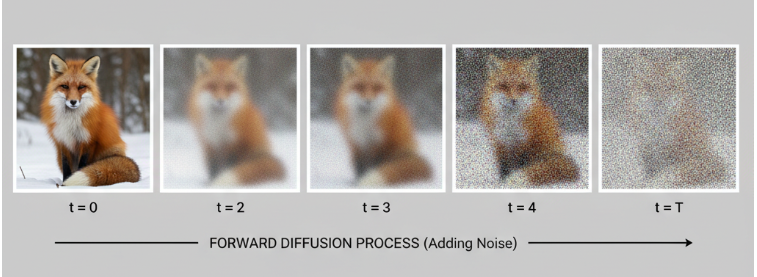
I begin with a simple experiment that shows how an input changes its distribution as Gaussian noise is added step by step, using the formula introduced in the DDPM paper (Denoising Diffusion Probabilistic Models, Jonathan Ho, Ajay Jain, Pieter Abbeel):
\[X_t = \sqrt{\bar{\alpha}_t} \, X_0 + \sqrt{1 - \bar{\alpha}_t} \, \tilde{\epsilon}, \quad \tilde{\epsilon} \sim \mathcal{N}(0,1)\]Experiment Setup
I repeated this for several timesteps:
\[t = 0, 20, 50, 80, 100, 300, 700, 999 \quad (\text{out of } 1000)\]For each noisy version $X_t$, I plotted:
- The noisy image.
- The histogram of its pixel values.
- The mean and variance of the pixel distribution.
Results
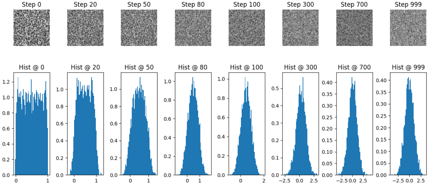
Step 0: mean = 0.4992, variance = 0.0845
Step 20: mean = 0.4965, variance = 0.0900
Step 50: mean = 0.4917, variance = 0.1123
Step 80: mean = 0.4775, variance = 0.1497
Step 100: mean = 0.4689, variance = 0.1760
Step 300: mean = 0.3067, variance = 0.6441
Step 700: mean = 0.0609, variance = 0.9867
Step 999: mean = 0.0053, variance = 0.9665
Observations
- The image gets progressively noisier as we increase the timesteps.
- The pixel histograms spread out and move closer to a Gaussian distribution.
- By the final timestep, the image is almost pure Gaussian noise with mean close to $0$ and variance close to $1$.
Next Steps
The derivation of the math for the forward diffusion process is included below.
👉 The full experiment code is available on my GitHub.
Formula Derivation
Initial Setup
Let $X_0$ be the initial data. We assume:
\[X_0 \sim \mathcal{N}(\mu, 1)\]That is, $X_0$ follows a normal distribution with mean $\mu$ and variance $1$.
Ideally, we want $X_0$ to follow a normal distribution with mean $0$ and variance $1$.
In diffusion models, the forward process gradually adds noise to data over several timesteps.
At each step, we take the previous state and inject a small amount of Gaussian noise.
Formally, we define a sequence of random variables:
\[X_0, X_1, X_2, \dots, X_t\]where $X_0$ is the original data and each subsequent $X_t$ is obtained by adding noise.
Naive approach: adding noise directly
Suppose we add Gaussian noise $epsilon$ at each step:
\[X_1 = X_0 + \epsilon, \quad \epsilon \sim \mathcal{N}(0,1)\]If we repeat this step, we get:
\[X_2 = X_1 + \epsilon_2, \quad \epsilon_2 \sim \mathcal{N}(0,1)\]and so on, until $X_t$.
At the very first step, the variance becomes:
\[\mathrm{Var}(X_1) = \mathrm{Var}(X_0) + \mathrm{Var}(\epsilon) = 1 + 1 = 2\]At the next step:
\[\mathrm{Var}(X_2) = \mathrm{Var}(X_1) + \mathrm{Var}(\epsilon_2) = 2 + 1 = 3\]By repeating this process, the variance grows linearly with the number of steps.
Why is this a problem?
Such a rapid growth in variance causes the signal to be overwhelmed by noise too quickly.
This makes the forward process unstable and prevents the model from learning a meaningful reverse process.
To avoid this, we need a variance scheduler that controls how much noise is added at each step.
Instead of adding full unit-variance noise every time, we add only a small fraction, gradually increasing the variance over many steps.
Variance Scheduler
To control variance growth, we introduce a variance scheduler $\beta_t$:
- $\beta_t$ defines how noise changes over time (linear, cosine, or other schedules).
- Typically, $\beta_t$ is very small (e.g., 0.0001 to 0.02) so that noise is added gradually.
We now want the noise to satisfy:
\[\epsilon \sim \mathcal{N}(0, \beta_t)\]and
\[X_1 = X_0 + \epsilon\]Scaling the Components
We introduce constants $(a, b \in \mathbb{R})$ to scale the contribution of the previous sample and the noise:
\[X_1 = a X_0 + b \epsilon\]where $(\epsilon \sim \mathcal{N}(0,1))$.
Finding (b)
We want the noise term to contribute variance $(\beta_t)$.
Currently, since $(\epsilon \sim \mathcal{N}(0,1))$, its variance is 1.
To scale it properly, we set:
so that
\[\text{Var}(b \epsilon) = \text{Var}(\sqrt{\beta_t} \ \epsilon) = \beta_t \cdot \text{Var}(\epsilon) = \beta_t\]Thus:
\[b = \sqrt{\beta_t}\]Forward Diffusion Step
Thus, the properly scaled forward diffusion step is:
\[X_1 = a X_0 + \sqrt{\beta_t} \ \epsilon, \quad \epsilon \sim \mathcal{N}(0,1)\]- $a$ scales the contribution of the previous sample.
- $\sqrt{\beta_t} \ \epsilon$ adds noise with the correct variance.
This ensures the variance increases gradually as noise is added.
Finding $a$
Now, we want $\text{Var}(X_1) = 1$.
\[\begin{aligned} \text{Var}(X_1) &= \text{Var}(a X_0 + \sqrt{\beta_t} \, \epsilon) \\ &= a^2 \, \text{Var}(X_0) + \beta_t \, \text{Var}(\epsilon) \\ &= a^2 \cdot 1 + \beta_t \cdot 1 \\ &= a^2 + \beta_t \end{aligned}\]To keep the variance at $1$:
\[a^2 + \beta_t = 1 \quad \implies \quad a = \sqrt{1 - \beta_t}\]So the update becomes:
\[X_1 = \sqrt{1 - \beta_t} \, X_0 + \sqrt{\beta_t} \, \epsilon\]General Case
In the general case, the forward diffusion process is:
\[X_t = \sqrt{1 - \beta_t} \, X_{t-1} + \sqrt{\beta_t} \, \epsilon_t, \quad \epsilon_t \sim \mathcal{N}(0,1)\]Introducing $\alpha_t$ and Cumulative Product
To compute the final data directly, It is common to define:
\[\alpha_t = 1 - \beta_t\]We also define the cumulative product of $\alpha_t$:
\[\bar{\alpha}_t = \prod_{s=1}^{t} \alpha_s\]This represents the total retained signal from the original data $X_0$ after $t$ steps.
Closed-Form Expression for $X_t$
Using the cumulative product, we can write $X_t$ in closed form using recursion: :
\[X_t = \sqrt{\bar{\alpha}_t} \, X_0 + \sqrt{1 - \bar{\alpha}_t} \, \tilde{\epsilon}, \quad \tilde{\epsilon} \sim \mathcal{N}(0,1)\]This formula is extremely convenient because it allows us to sample $X_t$ directly without iterating through all the intermediate steps.