Building a Tic Tac Toe Agent with Proximal Policy Optimization
Setting up the Tic Tac Toe Environment
I needed to create an environment that simulates Tic Tac Toe. I used a 3×3 NumPy array to represent the board:
0means the cell is empty.1means the agent (X).-1means the opponent (O).
The environment takes an action (which cell to put an X in), updates the board, then the opponent makes a random valid move. I also programmed it to check for wins, losses, draws, or invalid moves.
Here’s how the empty board looks initially:
Initial State:
[[0 0 0]
[0 0 0]
[0 0 0]]
When I took an action (for example, placing an X in cell 1), the board updated like this:
State after taking action 1:
[[0 1 0]
[0 0 0]
[0 0 0]]
The Actor-Critic Neural Network
To teach the agent how to play, I built a neural network with an Actor-Critic architecture. The network does two things:
- The actor picks the next move.
- The critic estimates how good the current board state is (the expected return).
I fed the board (flattened into 9 numbers) into the network. The actor outputs scores (called logits) for each possible move, but since some cells might be taken, I masked out invalid moves so the agent never chooses them.
Here’s an example output from the network before training:
Selected action: 1 Log probability: -2.20 Entropy: 2.20 Value estimate: 0.007
This shows the network’s initial guess, the uncertainty in its choice, and how it values the current board.
How PPO Helps the Agent Learn
Proximal Policy Optimization (PPO) tweaks the agent’s policy (its way of choosing moves) gently, avoiding big changes that can destabilize learning. It does this by clipping how much the policy can update based on advantages — basically how much better a move turned out than expected.
I also used Generalized Advantage Estimation (GAE) to compute smoother advantage values, balancing bias and variance.
PPO and GAE Equations
-
Temporal Difference (TD) Residual: \(\delta_t = r_t + \gamma V(s_{t+1}) - V(s_t)\)
-
Generalized Advantage Estimation (GAE): \(\hat{A}_t = \delta_t + \gamma \lambda (1 - d_t) \hat{A}_{t+1}\)
or equivalently: \(\hat{A}_t = \delta_t + (\gamma \lambda)\delta_{t+1} + (\gamma \lambda)^2\delta_{t+2} + \cdots + (\gamma \lambda)^{T-t-1}\delta_{T-1}\)
-
Return Estimate for Value Function: \(R_t = \hat{A}_t + V(s_t)\)
-
PPO Clipped Objective: \(L^{\text{CLIP}}(\theta) = \hat{\mathbb{E}}_t \left[ \min \Big( r_t(\theta)\hat{A}_t,\; \text{clip}(r_t(\theta), 1 - \epsilon, 1 + \epsilon)\hat{A}_t \Big) \right]\)
where the probability ratio is: \(r_t(\theta) = \frac{\pi_\theta(a_t | s_t)}{\pi_{\text{old}}(a_t | s_t)}\)
Training the Agent
I trained the agent by letting it play many episodes against a random opponent.
After each episode, I gathered data about states, actions, rewards, and estimated values. Then I computed advantages and returns using GAE. Finally, I updated the neural network using the PPO loss function.
Here’s a snippet of the training progress where I evaluated the agent’s win rate every 100 iterations:
| Iteration | Win Rate |
|---|---|
| 100 | 0.30 |
| 200 | 0.45 |
| 300 | 0.60 |
| … | … |
Slowly but surely, the agent learned to win more often!
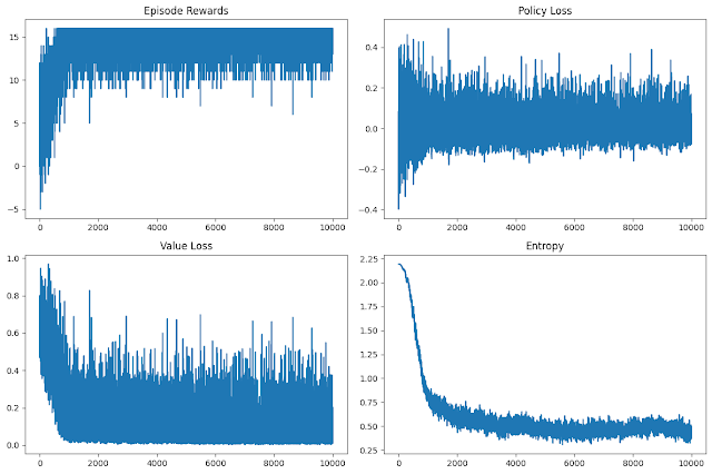
Fig: Training Loss, Rewards, Entropy
Playing Against My Agent
Once trained, I added a simple interface to play against the agent myself. Here’s a sample interaction:
…
Your move (0–8): 4
Agent moves…
X . .
. O .
. . .
I enter a move by typing a number from 0 to 8 (mapping to board cells), then the agent makes its move. This was a fun little project that I did on my vacation. I got my hands dirty with reinforcement learning, and it was really interesting. :) ```